


Filamentous networks and elastic polymers immersed in a viscous fluid are central to many processes in biology. Here, we present a model of a discrete viscoelastic network coupled to a Stokesian fluid. The network is built out of a collection of cross-linked nodes where each link is modeled by one or more simple viscoelastic elements. The method of regularized Stokeslets is used to couple network dynamics with a highly viscous fluid in three dimensions. We use computational rheometry tests to characterize the viscoelastic structures, such as computing their frequency-dependent loss and storage moduli. We find that when linkages between nodes are modeled by Maxwell elements, the qualitative behavior of these moduli reflects that of many biological viscoelastic structures.
I. INTRODUCTION
Elastic polymers and filamentous networks immersed in a fluid environment are ubiquitous in biology. For successful fertilization, a mammalian sperm must first penetrate two concentric layers of such viscoelastic networks. Figures 1(a) and 1(b) show the outermost layer, which contains cumulus cells bound together by an elastic matrix and the innermost layer, the zona pellucida (ZP). The ZP is a glycoprotein layer which contains ligands that bind to receptors on the sperm head, causing the sperm to release the enzymatic contents of its acrosome to facilitate penetration. Recent work has examined the viscoelastic properties of the ZP1,2 and the relative importance of propulsive forces from flagellar beating and biochemical binding forces in successful sperm-egg contact.3
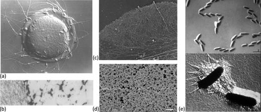
(a) Mouse oocyte surrounded by zona pellucida and sperm cells. Reprinted from P. M. Wassarman, “Contribution of mouse egg zona pellucida glycoproteins to gamete recognition during fertilization,” J. Cell. Physiol. 204, 388–391 (2005). Copyright 2005 Wiley-Liss, Inc.4 (b) Electron micrograph showing the zona pellucida and the extracellular matrix (ECM) of a hamster oocyte. Reprinted with permission from Talbot et al., “Motile cells lacking hyaluronidase can penetrate the hamster oocyte cumulus complex,” Dev. Biol. 108, 387–389 (1985). Copyright 1985 Elsevier.5 (c) Electron micrograph of actin network in a Xenopus fibroblast. Reprinted from T. M. Svitkina and G. G. Borisy, “Arp2/3 complex and actin depolymerizing factor/cofilin in dendritic organization and treadmilling of actin filament array in lamellipodia,” J. Cell Biol. 145, 1009–1026 (1999). Copyright 1999 Rockefeller University Press.6 (d) Electron micrograph showing network microstructure of lung mucus, reprinted with permission from Schuster et al., “Nanoparticle diffusion in respiratory mucus from humans without lung disease,” Biomaterials 34, 3439–3446 (2013). Copyright 2013 Elsevier.7 (e) Electron micrograph of bacteria and the extracellular polymeric substance (EPS) that the bacterian produce in the formation of a biofilm (JW Costerton archives, Center for Biofilm Engineering, Montana State University).
(a) Mouse oocyte surrounded by zona pellucida and sperm cells. Reprinted from P. M. Wassarman, “Contribution of mouse egg zona pellucida glycoproteins to gamete recognition during fertilization,” J. Cell. Physiol. 204, 388–391 (2005). Copyright 2005 Wiley-Liss, Inc.4 (b) Electron micrograph showing the zona pellucida and the extracellular matrix (ECM) of a hamster oocyte. Reprinted with permission from Talbot et al., “Motile cells lacking hyaluronidase can penetrate the hamster oocyte cumulus complex,” Dev. Biol. 108, 387–389 (1985). Copyright 1985 Elsevier.5 (c) Electron micrograph of actin network in a Xenopus fibroblast. Reprinted from T. M. Svitkina and G. G. Borisy, “Arp2/3 complex and actin depolymerizing factor/cofilin in dendritic organization and treadmilling of actin filament array in lamellipodia,” J. Cell Biol. 145, 1009–1026 (1999). Copyright 1999 Rockefeller University Press.6 (d) Electron micrograph showing network microstructure of lung mucus, reprinted with permission from Schuster et al., “Nanoparticle diffusion in respiratory mucus from humans without lung disease,” Biomaterials 34, 3439–3446 (2013). Copyright 2013 Elsevier.7 (e) Electron micrograph of bacteria and the extracellular polymeric substance (EPS) that the bacterian produce in the formation of a biofilm (JW Costerton archives, Center for Biofilm Engineering, Montana State University).
Cell cytoskeletons are built out of viscoelastic networks of biopolymers that provide the cell structure and shape. Polymerization of the actin network within a cytoskeleton also provides propulsive forces in ameboid cells and fibroblasts.8 Such an active network in a fibroblast is shown in Figure 1(c).6 Contaminating particles in the airways of the lung are cleared by mucociliary transport, where coordinated ciliary beating in the periciliary layer propel a mucus layer that traps the particles. Figure 1(d) shows the microstructure of respiratory mucus comprised of gel-forming mucins.7 Recent experiments suggest that the periciliary layer is not a simple Newtonian fluid, but is itself spanned by a network of mucins.9 Finally, Figure 1(e) shows an example of a bacterial biofilm. Here, we see individual bacterial cells adhered to a surface, surrounded by a self-produced network of extracellular polymeric substance (EPS). Rheometry has demonstrated that biofilms behave as viscoelastic polymeric fluids.10
In each of these examples, we observe a complex, spatially heterogeneous system where a network structure is coupled to a surrounding fluid. The dynamics of these heterogeneous systems will evolve due to the additional forces applied to the network-fluid system by external flows, the actuated flagella of the sperm or bacterial cells, the motion of the respiratory cilia, or the remodeling of the actin filaments due to polymerization. Our modeling efforts seek to capture the spatial heterogeneity of the system and the discrete microscale structure of the network. For this reason, we do not chose a continuum description of a viscoelastic fluid. Rather, we present a computational framework that couples forces due to the viscoelastic network to a surrounding viscous fluid in three-dimensions, governed by the Stokes equations. The viscoelastic model presented here is inspired by the work of Bottino11 and Dillon and Zhuo12 where forces due to a viscoelastic network are coupled to a two-dimensional Navier-Stokes fluid using an immersed boundary method. A related model of viscoelastic biofilm dynamics in three dimensions was also presented in Ref. 13. Because we are motivated by understanding viscoelastic networks at the microscale, here we choose a regularized Stokeslet formulation of the coupled system.14,15 In this way, we can exploit the existence of fundamental solutions and image solutions to account for a planar boundary.
The viscoelastic network is represented as a collection of nodes and connections. A connection between two nodes in the network satisfies an assigned constitutive law. While more complex stress-strain relationships may be used, here a connection is taken to be either a spring element or a spring and dashpot in series (Maxwell element). We will demonstrate that when forces from these elements are coupled to the Stokes equations, the surrounding viscous fluid acts as a dashpot in parallel with the element. In order to characterize the material properties of a network structure built out of these individual elements, we subject the structure to computational rheometry tests. We examine the results of a creep test, a relaxation test, and a small amplitude oscillatory shear (SAOS) test. For simplicity, here we consider regular network structures whose nodes are initialized on a rectangular lattice (see Figure 2). The material parameters of each individual element are taken to be fixed in time, as is the network topology. We remark that this modeling framework can readily incorporate dynamic elements, that are broken, for instance, if they get stretched beyond a certain threshold.

This paper is organized as follows. Section II introduces the basic linear viscoelastic elements and their known responses to standard rheological experiments. In Sec. III, we outline the governing equations that couple these viscoelastic elements to a viscous fluid. In Sec. IV, we examine the response of individual elements to rheological tests when they are immersed in a Stokesian fluid. In Sec. V, we perform the same rheological tests on a viscoelastic structure comprised of these individual elements. Finally, we show that this model does capture realistic viscoelastic behavior, and also present a computational micropipette aspiration test in three dimensions.
II. MECHANICAL MODELS FOR LINEAR VISCOELASTICITY
The simplest approach to characterize any viscoelastic material is to compare its elastic response to that of a simple mechanical model using linear elasticity. The (Young's) modulus of elasticity, E, of a material that obeys Hooke's law is defined as the ratio of stress to dimensionless strain, i.e., E = σ/ɛ. Since ɛ is dimensionless strain, the Young's modulus E has the same units as stress σ. For viscoelastic materials that exhibit the behavior of both viscous fluids and elastic solids, it is not sufficient to specify a single modulus. In this section, we briefly review some rheological tests and the known responses that basic viscoelastic elements display under a constant stress and when a constant or an oscillatory strain is applied.
A. Review of rheology
A rheological measurement is used to characterize a viscoelastic material.16–19 A rheometer measures the properties of a material based on its deformation, deformation rate, or frequency of deformation. Common rheological procedures used to characterize viscoelastic properties are the creep, stress relaxation, and small amplitude oscillatory shear tests, which we briefly describe below. In the stress relaxation and the small-amplitude oscillation tests, a given strain is imposed on the material and the resulting stresses are measured. Alternatively, in the creep test, a shearing stress is imposed and the resulting shearing strain is measured.
1. Creep test
We can measure the behavior of the viscoelastic material by applying a constant stress σ0 for a fixed time interval [t0, t1]
where H is the Heaviside function, and we compute the corresponding strain ɛ(t) — a creep function or simply a creep.
2. Stress relaxation test
A common way to measure the viscoelastic response of a material is by its stress relaxation. We apply an instantaneous displacement (strain) ɛ0 at time t0 to measure the stress response σ(t). Given ɛ(t) = ɛ0H(t − t0), the relaxation modulus G(t) is defined as
3. SAOS test
In this dynamic test, an oscillatory sinusoidal strain is applied to the viscoelastic material and the resulting stress is measured. The imposed strain function takes the form
where ω is the frequency of oscillations and ɛ0 is a dimensionless amplitude. Note that the strain rate,
and its amplitude increases with higher frequencies. The resulting stress, σ(t), will eventually reach a steady state in which it also oscillates sinusoidally at the same frequency but shifted in phase by an angle θ. The stress takes form σ(t) = σ0sin (ωt + θ), which is typically represented as
The term proportional to G′(ω) is in phase with the strain and is called the storage modulus, as it represents storage of elastic energy. The term G′′(ω) is in phase with the strain rate,
B. Basic linear viscoelastic models
Typical viscoelastic models are combinations of springs and dashpots connected in series or in parallel. The building blocks and their behavior in the rheological tests described earlier are shown in Figures 3(a) and 3(b). Note that a dashpot does not have any stress relaxation response since the element immediately opened stays open; there is no stress developed along the element and the relaxation modulus is zero for all time. Figure 3 also shows both two-element models, the Maxwell and Kelvin-Voigt models, and one three-element model, Fluid 1. Generally, we expect that more realistic materials are better modeled using more elements, which display more complex rheological behavior.
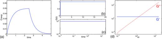
![FIG. 3. Linear elastic, viscous, and viscoelastic mechanical models with their creep functions, relaxation, storage, and loss moduli. (a) An elastic spring, Eɛ = σ, (b) a viscous dashpot, \documentclass[12pt]{minimal}\begin{document}$\eta \dot{\varepsilon }=\sigma$\end{document}ηɛ̇=σ, (c) Maxwell element, \documentclass[12pt]{minimal}\begin{document}$\eta E\dot{\varepsilon }=E\sigma +\eta \dot{\sigma }$\end{document}ηEɛ̇=Eσ+ησ̇, (d) Kelvin-Voigt element, \documentclass[12pt]{minimal}\begin{document}$E\varepsilon + \eta \dot{\varepsilon } =\sigma$\end{document}Eɛ+ηɛ̇=σ, and (e) Fluids 1 element, \documentclass[12pt]{minimal}\begin{document}$\eta _1\eta _2\ddot{\varepsilon } + E(\eta _1 + \eta _2)\dot{\varepsilon }= E\sigma + \eta _2\dot{\sigma }$\end{document}η1η2ɛ̈+E(η1+η2)ɛ̇=Eσ+η2σ̇.](https://aipp.silverchair-cdn.com/aipp/content_public/journal/pof/26/11/10.1063_1.4900941/1/m_113102_1_f3.jpeg?Expires=1716337417&Signature=BMD8F1kBXbVptLLXN1-o5p8FKoj9oJCOK-nRu20I1yolUNd0UdVi8BIgmwBbZ0Q70NkdkqNqABsVb3PvnTSEltzs4Y5dxYdaDS8E1RSNIpY2NsEUumiKLm-E82SvnKfXuosc0xUhaPlwiNbT87TSkplEZWmaklXO4hiYorDPVJmB8HbCG~t8HL1Y8a22lCBoIJr3KbA-EYN7VyrWklN0ZfhwqPBLBcFJtLSwASkzeOXZi5xKo6YLkhw5UACAf1Lq0ff0xQ7B4bZzSPlhmGoBlrWHVBjSBcDvUVjuYcl1dIFs1aif8VypIebmxjSoDRc6wNDSkIt6~5wcguCcFbrf4A__&Key-Pair-Id=APKAIE5G5CRDK6RD3PGA)
Linear elastic, viscous, and viscoelastic mechanical models with their creep functions, relaxation, storage, and loss moduli. (a) An elastic spring, Eɛ = σ, (b) a viscous dashpot,
Linear elastic, viscous, and viscoelastic mechanical models with their creep functions, relaxation, storage, and loss moduli. (a) An elastic spring, Eɛ = σ, (b) a viscous dashpot,
In the creep test, all elements react immediately upon applying a stress and some of them eventually return to their initial configuration after the stress is turned off. Other elements that have a dashpot in series, do not return to their initial configuration (see Figures 3(c) and 3(e)). We also note that the one- and two-element models are special cases of the three-element model by setting appropriate parameter values to zero. All of the models can be described in terms of a relation between stress and strain. The SAOS column shows the graphs of G′ and G′′ defined in Eq. (5) as a function of frequency. Captions of Figure 3 provide the constitutive relation for each element. Based on these relations, analytical formulas for the creep function, the relaxation, storage, and loss moduli can be derived and evaluated, for some initial conditions provided.20 Our goal is to describe the behavior of viscoelastic elements when they are immersed in a Stokesian fluid.
III. STOKES FLOW
We aim to understand the behavior of a viscoelastic material immersed in a fluid, where the material is represented by a collection of nodes connected by viscoelastic elements composed of springs and dashpots; see Figure 2. Since these elements will develop stresses that interact with the fluid, our model requires a way of determining the fluid motion due to forces, and also a way to evolve the viscoelastic network due to the fluid motion. For this we use the method of regularized Stokeslets,14,15 which we briefly describe next.
Motivated by microscopic phenomena, we assume the fluid motion is governed by the incompressible Stokes equations
where μ is the fluid viscosity, u is the fluid velocity, p is the pressure, and F is the external force per unit volume. The motion of a particle at location xi(t) immersed in the fluid satisfies the equation
To compute the motion of the fluid and any particle in the fluid, we use the method of regularized Stokeslets, where a force concentrated at a point xk is assumed to be given by F(x) = fkϕδ(x − xk), where fk is a vector force coefficient. The function ϕδ(x − xk) is bell-shaped, radially symmetric, with a maximum value at xk and integrates to one. The exact form of the function used here is
where rk = ‖x − xk‖. The parameter δ controls the width of the function. In the case of N forces (k = 1, 2, …, N), the Stokes equation with this type of forcing can be solved exactly using superposition to give
This method has been widely used to investigate low Reynolds number hydrodynamics in applications such as microorganism motility,15,21–24 biofilm dynamics,25,26 cancer cells in flow,27 microfiltration as a method for removing particulate matter,28 and to study hydrodynamic interactions that cause synchronization between rotating paddles in a viscous fluid.29
The inclusion of a rigid wall where the fluid velocity must satisfy the zero-flow boundary condition can be accomplished by using a method of images.30,31 In our context, the Stokeslets kernel is modified using the method described in Ref. 32, where other elements are placed at the mirror image of every node about the wall in such a way that the velocity contributions from the node Stokeslets and the additional elements at the node images is zero analytically at the wall.
The sum in Eq. (8) can be interpreted in two different ways. It may represent a superposition of velocity contributions from forces at scattered points, as is the case of the viscoelastic network in Figure 2. In other instances, the right side of Eq. (8) may represent a surface integral discretization. Depending on the interpretation of the formula, the regularization parameter δ may be chosen based on different criteria. We explain this in detail in Secs. IV and V G.
Because of the linear dependence of the velocity field on the forces, Eq. (8) evaluated at xj can be written into vector-matrix form
where Sj(x1, x2, …, xN) is a 3 × 3N matrix and
A. Dimensional analysis
Before we introduce a method for modeling viscoelastic elements or more complex structures immersed in viscous fluid we scale the problem using characteristic quantities. Variables without tilde are nondimensional, whereas all variables with tilde (e.g.,
We now choose a fluid viscosity μo to scale the pressure and forces, and set P = μoU/L and F = μoU/L2 to get the dimensionless equations
where μe = μ/μo and the regularization parameter
Then the SAOS equations become
where
and
IV. VISCOELASTIC ELEMENTS IMMERSED IN A STOKESIAN FLUID
We revisit the behavior of viscoelastic elements described in Figure 3 but in the context of being immersed in a Stokes flow, where the stresses developed by the elements affect the motion of the fluid surrounding them.
A. Stokes-null element
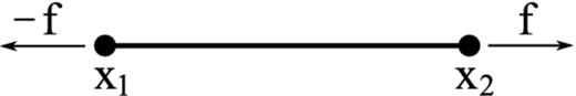
Since in the fluid medium, a force at one point affects the motion of other points in the fluid, we consider first a “null element” consisting of two points x1(t) and x2(t) in the fluid with no connection between them. When a constant force f is applied in opposite directions at the two endpoints, the “null element” extends; see Figure 4.
We calibrate the value of δ for the network nodes as follows. The Stokeslet velocity at point x2 from Eq. (8) produced by both forces located at x1 and x2 reduces to
so that if δ ≪ ‖x2 − x1‖, we may write 4πμeδu(x2) ≈ f. This coincides with the strain-stress relationship of a dashpot (in vacuum), where the strain rate of the element is proportional to the stress, i.e.,
Figure 5 shows the result of a creep test on the null element using the parameters δ = 1/4π and μe = 1. Two points, x1 and x2, are initially placed one unit apart. The points are not connected in any way. At time t0, equal and opposite forces (stress) of magnitude ‖f‖ = 0.05 are applied at those points moving them away from each other. At time t1 = t0 + 2.5, the forces are removed and the motion stops. Figure 5(a) shows the velocity field near the null element at the moment the forces are first applied. The separation between the element endpoints minus the initial separation is plotted in Figure 5(b), which shows the same rheological response as the dashpot in Figure 3(b). The increasing portion of the creep function has slope equal to ‖u2 − u1‖ = 2‖u2‖ ≈ 2‖f‖/4πμeδ = 2‖f‖ = 0.1. We conclude that the fluid environment has the damping effect of a dashpot connecting the two endpoints of the null element.

Acting forces (bold arrows) and velocity field around the Null element during a creep test, (a) at t0, the beginning of the loading phase of the test, (b) creep function for ‖f‖ = 0.05. The initial point separation is set to 1, δ = 1/4π, and μe = 1.
Acting forces (bold arrows) and velocity field around the Null element during a creep test, (a) at t0, the beginning of the loading phase of the test, (b) creep function for ‖f‖ = 0.05. The initial point separation is set to 1, δ = 1/4π, and μe = 1.
B. Stokes-spring element
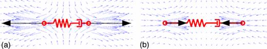
We consider now the two points x1(t) and x2(t) connected by a spring immersed in the fluid. We perform the creep test as before by applying a constant force f in opposite directions at the two endpoints, pulling them apart; see Figure 6.

In this case, the spring exerts a restoring force given by
where ℓ0 denotes the fixed spring resting length and E is the modulus of elasticity. As the element stretches due to the applied force f, the spring force fs increases until a time it balances the applied force at each endpoint. Upon removing this applied force f, the spring shrinks back to its initial length asymptotically in time due to the fluid damping. At any given time while f is applied, the net force at x1 is −f + fs(x1) and the net force at x2 is f + fs(x2). When f is removed, only the spring forces remain at the endpoints. With these forces, we use Eq. (8) to compute the velocities of the two element endpoints. Figure 7(a) shows the velocity field around the spring at the instant the force f is first applied; Figure 7(b) shows the velocity field at the instant f is removed.

Acting forces (bold arrows) and velocity field around the Stokes-spring element during a creep test, (a) at t0 and (b) at t1, the beginning of loading and unloading phase of the test, respectively.
Acting forces (bold arrows) and velocity field around the Stokes-spring element during a creep test, (a) at t0 and (b) at t1, the beginning of loading and unloading phase of the test, respectively.
The creep function for the spring element is element length minus its length at t = 0 and is shown in Figure 8(a). The force f is applied at t = 0 and removed at t = 2.5. Notice that it resembles the creep function for the Kelvin-Voigt element in Figure 3(d), which is consistent with the notion that the viscous fluid acts as a dashpot in parallel with the spring element.
Stokes-spring element with E = 1, ℓ = 1, ɛ0 = 0.1; μe = 1 and δ = 1/4π and an initial length 1: (a) creep function for ‖f‖ = 0.05, (b) relaxation modulus and (c) its log-log plot, (d) storage and loss moduli.
Stokes-spring element with E = 1, ℓ = 1, ɛ0 = 0.1; μe = 1 and δ = 1/4π and an initial length 1: (a) creep function for ‖f‖ = 0.05, (b) relaxation modulus and (c) its log-log plot, (d) storage and loss moduli.
In the stress relaxation test, the spring is instantaneously stretched beyond its resting length and kept at that separation by applying a force f which exactly balances the spring force at each endpoint of the element. Since the applied force f is constant, so is the relaxation modulus G(t) shown in Figures 8(b) and 8(c). These two also look exactly like those for the Kelvin-Voigt model.
Next, we perform the SAOS test introduced in Sec. II A. The test consists of applying a sinusoidal strain ɛ(t) given by Eq. (3) to the right end of the spring element and −ɛ(t) at the left end. Since the element length is known and given by 2ɛ(t), the spring force fs(t) is readily computed from Eq. (10). The only unknown is the force f(t) that must be applied at the endpoints in order to maintain the desired sinusoidal strain. This force is computed from the regularized Stokeslets formula in Eq. (9) by setting
which is a linear system that can be solved for the unknown force f. This applied force is used to compute the viscoelastic moduli as follows. The force f also oscillates sinusoidally at the same frequency as the imposed strain but shifted in phase. Using Eq. (5), we compute the storage and loss moduli G′ and G′′ by the decomposition
where e1 is the unit vector along the element axis. The computed values of G′ and G′′ are shown in Figure 8(d). As expected, the results resemble those of the Kelvin-Voigt model in which the dashpot in parallel with the spring has parameter η ≈ μe.
C. Stokes-Maxwell element
We consider one final type of element, a Maxwell element immersed in a fluid. This element consists of a spring and a dashpot in series; however, in our model we seek to represent this element simply as a spring with resting length that changes according to the stresses at the endpoints; see Figure 9.

When the element is stretched beyond its resting length, the dashpot opens so that the spring force is reduced. We motivate the evolution of the element resting length by considering the stress-strain relationship for a dashpot,
Simplifying and using the expression for the spring force in Eq. (10), we get
where x1(t) and x2(t) are the two endpoints of the element. Note that for η → ∞ Eq. (13) gives a constant resting length and it retrieves the Stokes-spring element introduced above.
In the creep test, we apply equal and opposite forces f at the endpoints, which stretches the spring. The spring force begins to counteract the applied force but the resting length begins to increase, thus the spring force is never large enough to cancel the applied force. Once f is removed, the spring force reduces the element length until it reaches an equilibrium at a resting length that is larger than ℓ0. The velocity field around the element at two different times during the creep test is shown in Figure 10. The creep function for the element, shown in Figure 11(a), looks like that of the Fluid 1 model in Figure 3(e) which consists of a Maxwell element in parallel with a dashpot. Here, again, the effect of the fluid viscosity is to act as a dashpot in parallel with the immersed element.
Acting forces (bold arrows) and velocity field around the Stokes-Maxwell element during a creep test, (a) at t0 and (b) at t1, the beginning of loading and unloading phase of the test, respectively.
Acting forces (bold arrows) and velocity field around the Stokes-Maxwell element during a creep test, (a) at t0 and (b) at t1, the beginning of loading and unloading phase of the test, respectively.

Stokes-Maxwell element with E = 1, η = 5, ℓ(0) = 1, ɛ0 = 0.1; μe = 1 and δ = 1/4π and an initial length 1: (a) creep function with σ0 = 0.05, (b) relaxation modulus and (c) its log-log plot, (d) storage and loss moduli.
Stokes-Maxwell element with E = 1, η = 5, ℓ(0) = 1, ɛ0 = 0.1; μe = 1 and δ = 1/4π and an initial length 1: (a) creep function with σ0 = 0.05, (b) relaxation modulus and (c) its log-log plot, (d) storage and loss moduli.
In the stress relaxation test, the element is stretched instantaneously to a fixed length and kept at that separation. As the resting length increases, the spring force fs decreases to zero asymptotically in time. The relaxation modulus G(t), computed as
In the SAOS test, the computed storage and the loss moduli G′, G′′ are evaluated as before by formula (12). The moduli for different frequencies of the strain oscillations are shown in Figure 11(d). The results resemble a Maxwell element in parallel with a dashpot due to the viscous fluid, i.e., the Fluid 1 element shown in Figure 3(e).
V. VISCOELASTIC NETWORK IMMERSED IN A STOKESIAN FLUID
In general, biological fluids exhibit both viscous and elastic behavior17 due to the fluid viscosity and the elastic or viscoelastic microstructures. Those microstructures can flow in the ambient fluid or remain attached to the wall creating elastic scaffolds. We focus on the second case where the structure is attached to a wall. Our model of a viscoelastic network in Figure 2 is comprised of nodes that are connected by one or more viscoelastic elements described above. We now describe computational rheometry tests that simulate a parallel-plate device that consists of fixed bottom plate and sliding top plate. A stress (strain) is applied to the top plate so that it moves horizontally and the resulting strain (stress) is measured. In this case, the stress σ is the force applied per unit area of the top plate and the strain ɛ is the horizontal displacement of the top plate divided by the gap between the plates.
In order to test the properties of a viscoelastic structure, we define the equilibrium position of a sample network using uniformly spaced nodes in a regular pattern occupying a rectangular slab of a cube, sitting on a planar wall located at z = 0; see Figure 2. The network node i at time t is denoted by xi(t). Each inner point of the network is connected by a link to its 26 closest neighbors. If xi(t) and xj(t) are connected, the resting length of the link joining them is denoted by ℓij(t). When stress or strain is imposed on the top layer of the structure, the links deform and forces develop at the nodes. Since the structure is attached to a planar wall, in simulations below we use regularized Stokeslets with images.32 The dynamics of the network evolve by requiring the nodes to move with the local fluid velocity induced by the forces at all the nodes (Eq. (7)).
The network, at equilibrium in Figure 2, is placed within a computational sliding plate rheometer. The connections between nodes are either Stokes-spring elements or Stokes-Maxwell elements. For simplicity, in each case the stiffness and damping coefficients of individual elements are the same for every connection. In the equilibrium configuration, all forces are zero. Once the nodes move, due to either an imposed stress or strain, the force at node xi(t) is given by
where xj's are all neighbor nodes connected to xi, Eij is stiffness constant and ℓij(t) is the resting length of the spring between node xi and xj that satisfies the relation (13) for the Stokes-Maxwell elements. It is constant in time, ℓij(t) = ℓij, 0, for the Stokes-spring elements.
The network forces are computed using Eq. (14). For the creep test, a constant stress is first applied to the top plate. We represent the imposed stress as a uniform distribution of force per area at the nodes anchored to the top plate. Once the stress is released, the system is driven only by the elastic forces of the network. In the two other tests, we impose the strain of the rheometer. For the relaxation test, a constant strain (displacement) is applied instantaneously (zero strain rate) while for SAOS the oscillatory strain from Eq. (3) is applied (strain rate in Eq. (4)). Since the strain rates of the top plate are known in both cases, the unknown forces along the top plate that are required to achieve these prescribed strain rates can be computed by solving a linear system based on Eq. (9). We do this using the GMRES33 iterative method with tolerance 10−12. The forces on the top plate initiate the motion of the entire network, which develops forces given by Eq. (14). The combination of all forces generates flow around the structure. At each time step, we evaluate the velocity at the discrete nodes from Eq. (8) and update their position based on the time-dependent Eq. (7), which is approximated with a fourth-order Runge-Kutta method with time step Δt = 10−3 for all creep simulations and Δt = 10−2 for all relaxation tests. For each specific frequency of oscillation ω in the SAOS tests, we ran the rheometer for two periods of oscillation (4π/ω) with 5 × 10⁴ time steps per period.
A. Creep tests
Under a constant stress applied to the top plate in a direction parallel to the wall, the equilibrium network in Figure 2 deforms as the top plate slides. The first row of Figure 12 shows snapshots of a Stokes-spring network at time t1 (panel (a)), the time of maximal distension when the stress on the top plate has been released, and then at the end of the test (panel (b)). In this case, we see that when the stress is removed, all springs in the network eventually relax back to their equilibrium resting lengths. The second row of Figure 12 shows snapshots of a Stokes-Maxwell network also at time t1 (panel (c)), the time of maximal distension when the stress on the top plate has been released, and at the end of the test (panel (d)). Here, we see that the Stokes-Maxwell network did not relax back to its initial configuration because of the dashpot components on the individual elements.
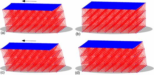
Discrete viscoelastic network comprised of an 8 × 8 × 4 lattice of nodes and connections with spacing h = 1 immersed in a viscous fluid and attached to a wall subjected to a creep test. (a) Stokes-spring network at time t1, the time of maximal distension when the stress on the top plate has been released, (b) Stokes-spring network at end of creep test, (c) Stokes-Maxwell network at time t1, the time of maximal distension when the stress on the top plate has been released, and (d) Stokes-Maxwell network at the end of the test.
Discrete viscoelastic network comprised of an 8 × 8 × 4 lattice of nodes and connections with spacing h = 1 immersed in a viscous fluid and attached to a wall subjected to a creep test. (a) Stokes-spring network at time t1, the time of maximal distension when the stress on the top plate has been released, (b) Stokes-spring network at end of creep test, (c) Stokes-Maxwell network at time t1, the time of maximal distension when the stress on the top plate has been released, and (d) Stokes-Maxwell network at the end of the test.
The creep function for each network is computed as
where P is the gap between the plates, N is the total number of nodes in the top plate, and

Creep functions for the link-node system attached to the wall subject to the step-function shear stress Eq. (1) with σ0 = 1, t0 = 0, and t1 = 0.5 with stiffness E = 10, E = 20, E = 40, respectively. (a) Response of the Stokes-spring network. (b)–(d) Response of the Stokes-Maxwell networks with damping constants η = 160, η = 40, and η = 10, respectively. In each case, μe = 1 and δ = 1/4π.
Creep functions for the link-node system attached to the wall subject to the step-function shear stress Eq. (1) with σ0 = 1, t0 = 0, and t1 = 0.5 with stiffness E = 10, E = 20, E = 40, respectively. (a) Response of the Stokes-spring network. (b)–(d) Response of the Stokes-Maxwell networks with damping constants η = 160, η = 40, and η = 10, respectively. In each case, μe = 1 and δ = 1/4π.
Figure 13(a) shows the results for the Stokes-spring network. In these cases, the creep function approaches zero at large times indicating that all connections eventually return to their original length. The distortion of the network decreases as the spring stiffness E increases, and the maximum value of the creep function also decreases as the stiffness E increases. The creep functions for the Stokes-spring network are qualitatively equal to those of a single Stokes-spring in Figure 8(a) and for the Kelvin-Voigt element in Figure 3(d).
Figures 13(b) and 13(d) present the creep functions for the Stokes-Maxwell network. Based on Eq. (13), we expect the spring resting lengths to adjust more slowly as η increases, leading to smaller network final deformations compared to their initial node positions when η is large. On the other hand, when η is small, the resting lengths adjust quickly to the imposed stress, keeping the springs continuously near equilibrium. Figure 13(d), for example, shows that when η is small, the resting lengths have increased so much by the time the stress is released that the network relaxes significantly less in time. For very small η, the dynamics resemble that of a Stokes-null element. Overall, the results show that the Stokes-Maxwell network elements can simulate a variety of material properties based on the choice of parameters.
B. Stress relaxation tests
In the stress relaxation test, we instantaneously displace the top plate horizontally from its equilibrium position by an amount h, equal to the spacing between nodes. We then hold the plate fixed at that position and measure the average magnitude of the resulting stress on the top plate. We do this by computing the spring forces at all nodes of the top plate, summing them, and dividing the result by the area of the plate. We use Eq. (2) with an initial plate displacement ɛ0 = h to compute the relaxation modulus G(t).
The relaxation modulus for the Stokes-spring network is shown in Figures 14(a) and 14(b), in linear and log-log scales, respectively. Although we have already seen a single spring immersed in a viscous fluid behave like a Kelvin-Voigt element, Fig. 8(b), the network behavior is slightly different. Figure 14(a) shows that after an instantaneous jump to a maximum value of G(t) when the strain is applied, the relaxation modulus does not stay at that value. Instead, it decreases exponentially to some nonzero value. The initial behavior of the modulus is more complex than that of any viscoelastic element. The reason is that the initial jump reflects the forces that develop on the top plate due to the instantaneous strain, but the rest of the network takes time to reach a steady state as the nodes move through the fluid. As the nodes below the top plate move, they affect the forces on the top plate nodes. After this initial network reconfiguration, the relaxation modulus approaches a nonzero constant, exactly like that for single element.

(a) Relaxation modulus for the Stokes-spring network, (b) its log-log plot, (c) relaxation modulus for the Stokes-Maxwell network, (d) its log-log plot. Here, E = 10, η = 10, ɛ0 = h = 1, μe = 1, δ = 1/4π.
(a) Relaxation modulus for the Stokes-spring network, (b) its log-log plot, (c) relaxation modulus for the Stokes-Maxwell network, (d) its log-log plot. Here, E = 10, η = 10, ɛ0 = h = 1, μe = 1, δ = 1/4π.
The same relaxation test was performed on the Stokes-Maxwell network with η = 10 and the results shown in Figures 14(c) and 14(d). After an initial spike, the relaxation modulus decays to zero exponentially, similar to several of the elements depicted in Figure 3 including the Fluid 1 element.
C. Small amplitude oscillatory shear test
In this test, the plate at the top of the network is subjected to a small amplitude oscillatory strain. After a transient period, the entire structure oscillates back and forth. We compute the stress by first finding the force f as discussed following Eq. (11) and dividing that total force on the top plate by its area. A three-dimensional stress is developed. The tangential stress in the shear direction oscillates with the same frequency as the input strain, whereas the other component of the tangential stress is zero. The normal stress also oscillates, but with doubled frequency. The oscillation of the normal stress is, however, about a magnitude smaller than that of the tangential stress; see Figure 15.
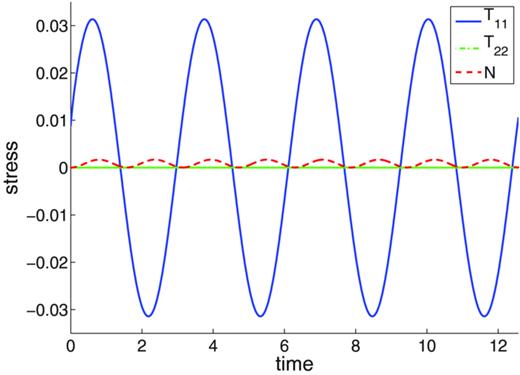
The top plate stress components measured during the SAOS test with frequency of oscillation ω = 2 and amplitude ɛ0 = 0.1, μe = 1, and δ = 1/4π.
The top plate stress components measured during the SAOS test with frequency of oscillation ω = 2 and amplitude ɛ0 = 0.1, μe = 1, and δ = 1/4π.
In order to compute the storage and loss moduli, we use Eq. (12) based upon the tangential stress measurements in the shear direction only. Figure 16(a) shows the moduli for the Stokes-spring network with E = 10. The results again resemble the single Stokes-spring element in Figure 8(b) or that for the Kelvin-Voigt element in Figure 3(d). Figures 16(b)–16(d) show the moduli for the Stokes-Maxwell network for different values of the damping constant η and fixed stiffness E = 10. We note that the storage modulus G′ tends to a constant at large frequencies and that this region of constant G′ begins at earlier frequencies when η is larger (compare panel (b) and panel (d)). Figures 16(b)–16(d) show that when Stokes-Maxwell elements comprise the network, the loss modulus G′′ develops a plateau region, where it is not monotonically increasing, for some range of frequencies. This is typical of viscoelastic biofluids such as mucus,34–36 DNA solutions,37 actin networks,38 and the intranuclear region of somatic cells.39 Finally, we note that the Stokes-spring network does not exhibit this plateau behavior. The loss modulus G′′ grows linearly whereas the storage modulus G′ is nearly constant for all frequencies; there is no frequency interval with plateau behavior of both moduli.
D. Viscoelastic link-node system of a different topology
In Secs. V A–V C, we performed rheological tests on a viscoelastic network whose nodes were placed uniformly on a rectangular lattice, and each internal node was connected to its 26 closest neighbors. Here, we investigate the dependence of the rheology of the slab of material on the network configuration by incorporating connectivity based upon a body-centered-cubic topology. The same uniformly spaced node distribution is used, but an additional node is placed at the center of each subcube. Moreover, each internal node of the lattice is connected to only its 14 nearest neighbors; see Figure 17(a).
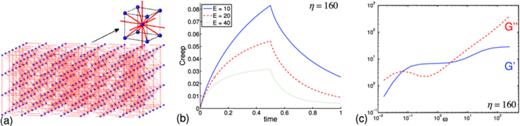
(a) Viscoelastic link-node system of the body-centered cubic topology, (b) creep functions for the Stokes-Maxwell system with damping constants η = 160 and with stiffness E = 10, E = 20, E = 40, respectively, (c) storage and loss moduli for the system with E = 10, μe = 1, and δ = 1/4π.
(a) Viscoelastic link-node system of the body-centered cubic topology, (b) creep functions for the Stokes-Maxwell system with damping constants η = 160 and with stiffness E = 10, E = 20, E = 40, respectively, (c) storage and loss moduli for the system with E = 10, μe = 1, and δ = 1/4π.
We repeat the same set of creep and SAOS tests using the same material parameters. The creep functions for the body-centered-cubic lattice shown in Figure 17(b) are qualitatively similar to those for the regular lattice (Figure 13(b)). The magnitude of the creep functions in the body-centered-cubic case is slightly larger due to fewer links between the top plate and the network.
Similarly, the storage and loss moduli computed in the SAOS tests for each network are similar (compare Figure 17(c) and Figure 16(b)). The magnitude of the storage modulus in the body-centered-cubic case is smaller since the structure is less stiff close to the oscillating plate. In this example, we see that the change in network topology does not have a big effect on the rheology of the material.
E. Comparison with measurements of storage and loss moduli of cytoskeleton networks
As it is our intention to apply this model of viscoelastic networks in Stokes flow to biological systems, we compare the storage and loss moduli computed for our simple network with measurements of such moduli of cytoskeletal networks.40,41 The cell's cytoskeleton is made up of filamentous proteins that provide a structural framework to the cell. Kole et al.40 use intracellular microrheology (ICM) to compute frequency-dependent viscoelastic moduli. Here, fluorescent nanoprobes are introduced, and then the statistical analysis of their motion allows the extraction of the local mechanical properties. Although our computational rheometry measurements of frequency-dependent viscoelastic moduli are completely different from this method of ICM, we may, nevertheless, examine the correspondence between the moduli for different choices of our network parameters. Figure 18(a) shows the storage and loss moduli computed using experimental data and ICM on human umbilical vein endothelial cells.41 Returning to dimensional units, Figure 18(b) shows that for a Stokes-Maxwell network as in Figure 2, the choice E = 5 Pa, η = 40 Pa s, T = 1 s, and fluid viscosity ten times that of water μ0 = 10−2 Pa s, the behaviours of the moduli are very similar to experiments.

(a) Storage and loss moduli of cytoplasm of human umbilical vein endothelial cells, G′(ω) (circles) and G′′(ω) (squares). Reprinted with permission from Panorchan et al., “Microrheology and ROCK signaling of human endothelial cells embedded in a 3D matrix,” Biophys. J. 91, 3499–3507 (2006). Copyright 2006 Elsevier.41 (b) Sample network of stiffness E = 5 Pa and viscosity η = 40 Pa s, results scaled by dimensional viscosity μo = 10−2 Pa s and time T = 1 s.
(a) Storage and loss moduli of cytoplasm of human umbilical vein endothelial cells, G′(ω) (circles) and G′′(ω) (squares). Reprinted with permission from Panorchan et al., “Microrheology and ROCK signaling of human endothelial cells embedded in a 3D matrix,” Biophys. J. 91, 3499–3507 (2006). Copyright 2006 Elsevier.41 (b) Sample network of stiffness E = 5 Pa and viscosity η = 40 Pa s, results scaled by dimensional viscosity μo = 10−2 Pa s and time T = 1 s.
F. Multiple elastic modes
A Boger fluid is a viscoelastic fluid whose viscosity is independent of shear rate.42 As such, elastic effects and shear effects can be clearly distinguished. For a typical Boger fluid, the loss modulus G′′ approaches a linear function of frequency ω as ω increases. The dynamic viscosity η′ of such a fluid is defined to be the slope of this line, i.e., η′ = G′′/ω. We find that the networks of Maxwell elements described above immersed in a Stokesian fluid exhibit features of Boger fluids (e.g., Figure 16(d)).
For a Boger fluid with multiple elastic modes, the storage and loss moduli are given by
Here, τi is a relaxation time, Ei is an elastic constant, and μ is the viscosity of the Newtonian solvent.43 Note the direct comparison with the storage and loss moduli for the Fluid 1 model in Figure 3(e)
For this single element, the relaxation time is τ = η1/E and the parallel dashpot constant η2 is analogous to the solvent viscosity.
In an effort to characterize the viscoelasticity of the fluid used in their experiments on helical swimming, Liu et al.43 assumed that, as in Eq. (15), the Boger fluid consisted of multiple elastic modes. Elastic constants and relaxation times were estimated by fitting experiments to these Oldroyd-B relationships. They assumed that the material was governed by the superposition of four relaxation times in Eq. (15) to match experimental data. The same approach was used by Baumgaertel and Winter in Ref. 44. We remark that the correspondence between a 2D viscoelastic discrete network model immersed in a fluid and an Oldroyd-B continuum model of a viscoelastic fluid was discussed in Ref. 12.
In our network model, the effects of multiple relaxation times can easily be modeled by considering multi-element links between nodes, with each link assigned its own elasticity and/or damping constant. For instance, consider the network in Figure 2 with each connection consisting of two Stokes-Maxwell elements with stiffness constants Ea = Eb = 10 and damping constants ηa = 10, ηb = 160. We subjected this network to the creep, relaxation, and SAOS tests. The creep function for the double network, Figure 19(a), shows that the structure is stiffer than those constructed with comparable single links in Figure 13. The stress relaxation modulus in Figures 19(b) and 19(c) shows that initially the structure relaxes rapidly, then like a faster relaxing network and next the relaxation modulus slows and decays like the network based on slowly relaxing elements. Macosko in Ref. 19 compares experimental relaxation modulus data with a single exponential model as well as a combination of a five-constant model with different relaxation constants, and shows that superposition of a few simple elements is necessary to match experimental data.
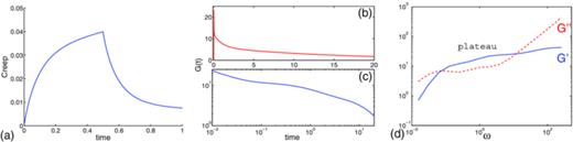
Double-linked Stokes-Maxwell network based on elements with Ea, b = 10, ηa = 10, and ηb = 160: (a) creep functions with σ0 = 1.0, (b) relaxation modulus for ɛ0 = 1.0, and (c) its log-log plot, (d) storage and loss moduli with solid and dashed line for ɛ0 = 0.1, μe = 1.0, and δ = 1/4π in all tests.
Double-linked Stokes-Maxwell network based on elements with Ea, b = 10, ηa = 10, and ηb = 160: (a) creep functions with σ0 = 1.0, (b) relaxation modulus for ɛ0 = 1.0, and (c) its log-log plot, (d) storage and loss moduli with solid and dashed line for ɛ0 = 0.1, μe = 1.0, and δ = 1/4π in all tests.
From the shape of storage and loss moduli, Figure 19(d), we can draw a few conclusions. We note that the relaxation time for the combined element (the first intersection of the moduli curves, τ = 1/ω) is close to the maximum relaxation time of the structure based on individual elements; compare with Figure 16(b) where E = 10 and η = 160. As ω → ∞, the storage modulus eventually approaches a constant value and the loss modulus approaches the same slope as those for the single-linked structures in Figure 16. Note that the storage and loss moduli for this double network exhibit long plateau behavior for certain range of frequencies even though the structures based on individual elements do not.
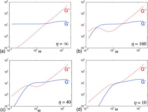
Log-log plot of ω vs. the storage and loss moduli for the shearing sinusoidal strain, Eq. (3) with the amplitude ɛ0 = 0.1, a stiffness constant for each element in the network is fixed at E = 10. (a) Moduli for the Stokes-spring network. (b)–(d) Moduli for the Stokes-Maxwell network: damping constant η = 160, η = 40, and η = 10, respectively. In each case, we use μe = 1 and δ = 1/4π.
Log-log plot of ω vs. the storage and loss moduli for the shearing sinusoidal strain, Eq. (3) with the amplitude ɛ0 = 0.1, a stiffness constant for each element in the network is fixed at E = 10. (a) Moduli for the Stokes-spring network. (b)–(d) Moduli for the Stokes-Maxwell network: damping constant η = 160, η = 40, and η = 10, respectively. In each case, we use μe = 1 and δ = 1/4π.
G. Micropipette aspiration test
Micropipette aspiration studies are often used to gain more information about the rheology of a viscoelastic material.2,45–47 We perform a computational micropipette aspiration test on a discrete viscoelastic network that is attached to a planar wall and immersed in a Stokesian fluid. The sample is constructed in a similar fashion as the structure introduced in Sec. V and is comprised either by Stokes-spring or Stokes-Maxwell elements.
A micropipette is modeled as a rigid cylinder with two open ends, one against the top layer of the network and the other high above the network. The setup consists of a solid wall at z = 0, a viscoelastic network occupying the (dimensionless) region {(x, y, z) : −1.4 ⩽ x ⩽ 1.4, −1.4 ⩽ y ⩽ 1.4, 0 < z ⩽ 0.6}, and a pipette of radius Rp = 0.5 and height Lp = 3.2 centered relative to the network (see Figure 20). In the simulation presented in this section, the cylindrical micropipette is discretized with 32 cross-sections and 32 points per cross-section, leading to a π/32 × 0.1 grid on the cylinder, or a linear discretization size of hp ≈ 0.1. The viscoelastic network is composed of 8 × 8 × 4 regularly spaced nodes, with the spacing between the nodes of h = 0.2, leading to a network height of H = 0.6.

Micropipette aspiration simulations at the sample mesh, links stiffness E = 10 and viscosity η = 5. Micropipette aspiration simulation with velocity field at time t = 0.5 for (a) Stokes-spring network and (b) Stokes-Maxwell network, respectively. (c) Creep function for the micropipette aspiration on both networks: relative aspiration length vs. time, sink strength 5.
Micropipette aspiration simulations at the sample mesh, links stiffness E = 10 and viscosity η = 5. Micropipette aspiration simulation with velocity field at time t = 0.5 for (a) Stokes-spring network and (b) Stokes-Maxwell network, respectively. (c) Creep function for the micropipette aspiration on both networks: relative aspiration length vs. time, sink strength 5.
In order to provide the suction, a single fluid sink is placed at the center of its circular cross section, close to the top end. An alternative formulation with a uniform low pressure at the top end of the pipette is also possible, but here we use a sink of strength s at x0 which produces a velocity field
The fluid velocity field has contributions from the sink, the network forces, and the surface forces on the micropipette. All of them are regularized elements with appropriate parameter δ. For the network forces, we use δ = h/4π, as discussed in Sec. IV. The sink regularization also uses the same value of δ as the network. The surface forces on the micropipette are different because their contribution to the velocity in Eq. (8) represents the discretization of a surface integral (with discretization size hp). Due to accuracy considerations of this integral approximation,15 we choose to regularize the pipette surface forces with δp = 0.1 ≈ hp. This fluid velocity is augmented by an image system in order to guarantee zero flow at the bottom wall.
At a given time in the computation, the network forces are computed using Eq. (14). These forces together with the sink induce a velocity field uw at the cylinder wall. In order to enforce zero flow at the pipette boundary, we solve a linear system using Eq. (9) for the pipette surface forces so that they induce a velocity that cancels uw at their location. The system is solved using the GMRES33 iterative method with tolerance 10−12. Once all forces are known, the fluid velocity at any location is computed using Eq. (8) plus the sink flow. The position of the discrete network nodes is updated using the fourth order Runge-Kutta method with time step Δt = 10−2. The full set of parameters used are summarized in Table I.
Set of parameters used in micropipette aspiration simulations.
| Parameter | Value |
|---|---|
| Network dimensions | [ − 1.4, 1.4]2 × [0, 0.6] |
| Network size, link length | 8 × 8 × 4, h = 0.2 |
| Network reg. parameter | δ = h/4π |
| Pipette radius | Rp = 0.5 |
| Pipette height | Lp = 3.2 (0.6 ⩽ z ⩽ 3.8) |
| Pipette patch | π/32 × 0.1 |
| Pipette reg. parameter | δp = 0.1 |
| Sink strength, location | s = 5, x0 = (0, 0, 3.25) |
At any time t, the aspiration distance is the maximum distance of any network node into the pipette. Figures 20(a) and 20(b) show snapshots of the aspiration deformation for the Stokes-spring network and the Stokes-Maxwell networks, respectively, along with the velocity field in the plane containing the axis of the pipette. The results of the creep test in Figure 20(c) show the response of the network under the aspiration simulations for both types of networks. The creep functions show similar behavior as for the sliding plate creep test in Figure 13.
Recently, Luo et al.48 used micropipette aspiration to study the effects of mechanical forces on cytoskeletal protein interactions and dynamic spatial localization of different proteins in the cortical network of an ameboid cell, Dictyostelium discoideum. For instance, it was observed that myosin II motors accumulated in the tip of the pipette, where the highest dilation of the cortical network occurs, and that greater applied pressure led to higher levels of accumulation. The cytoskeletal network of such an ameboid cell is an active network that can dynamically remodel itself due to the action of myosin motor proteins as well as spatial dynamics of other actin crosslinkers and anchoring proteins. In the simple case presented here, the network topology of the viscoelastic “cell” is static. However, we do see that the highest dilation of the network occurs in the pipette tip, as in the experiments. An extension of this numerical method would be to include a detailed model of cytoskeletal remodeling that does allow network topology to change in response to the dynamics of crosslinkers and motor proteins.
VI. DISCUSSION
Here, we have presented a model of viscoelastic networks coupled to a Stokesian fluid in three dimensions. These networks are built out of a collection of cross-linked nodes where each link is modeled by one or more simple viscoelastic elements. We have demonstrated that important features of viscoelastic networks, such as frequency-dependent loss and storage moduli, are captured when these structures are subjected to computational rheometry tests. We have also found that the background viscous fluid behaves as an additional dashpot in parallel with the viscoelastic elements. Moreover, we argue that linkages modeled only by springs as in the Stokes-spring networks, do not exhibit the plateau behavior of the loss and storage moduli measured for many viscoelastic biofluids such as mucus, actin networks, and DNA solutions. This behavior is captured when the linkages are modeled by Maxwell elements.
The strength of this modeling framework is that it readily couples the interaction of a surrounding fluid with both passive and actuated viscoelastic structures. Two-dimensional immersed boundary models based upon the full, incompressible Navier-Stokes equations and designed with similar goals, have been used to study sperm motility in viscoelastic media12 and cell-actin networks.11 The model presented here is fully three-dimensional, and because we assume the highly viscous flow of many biofluid dynamic systems, we are able to use the tools of Stokes flow such as image solutions and linearity. As illustrated in the micropipette example above, we can couple regions of Newtonian fluid with regions occupied by a viscoelastic fluid, as well as specify internal flow boundary conditions exactly, such as the zero flow on the boundary of the pipette.
For simplicity, we have considered simple networks whose nodes are initialized on a rectangular lattice and whose links are endowed with material parameters that are fixed in time. Moreover, the network topology is also fixed in time. Because of the discrete network formulation, this model may easily incorporate time-dependent material properties as well as dynamic elements between nodes that break or form based upon local network strains or stresses. In particular, we will use this numerical method to examine sperm penetration of the zona pellucida as well as ciliary transport of the mucus layer in the respiratory tract.
ACKNOWLEDGMENTS
The work of the authors was supported, in part, by the National Science Foundation (NSF) Grant No. DMS-104626. The authors thank Paula Andrea Vasquez for helpful discussions.

